Interaction With Matter
MSW Effect
Physics of MSW
As neutrinos passing by matter, the effective mass coming from energy change becomes important thus changing it’s eigenstates and propagation.
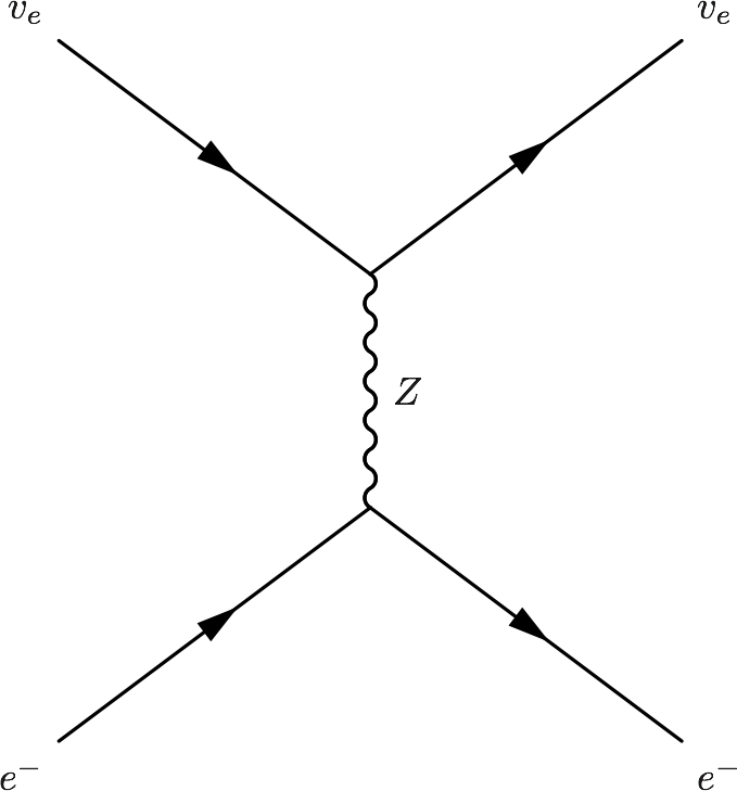
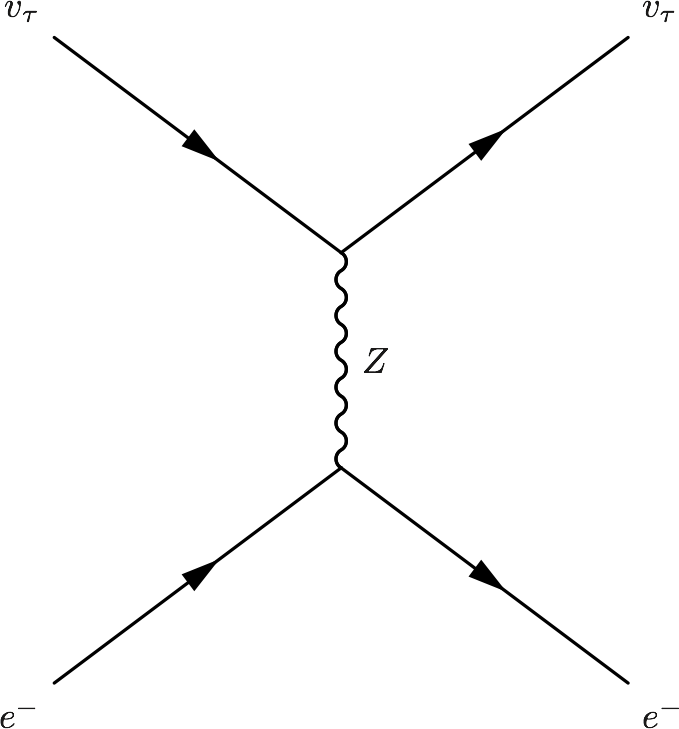
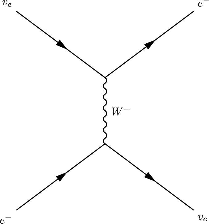
Neutrinos do interact with matter, mostly electrons in most cases.
\begin{fmfgraph*}(200,180)
  \fmfleft{i1,i2}
  \fmfright{o1,o2}
  \fmf{fermion}{i1,v1,o1}
  \fmf{fermion}{i2,v2,o2}
  \fmf{photon}{v1,v2}
  \fmflabel{$v_e$}{i2}
  \fmflabel{$e^-$}{i1}
  \fmflabel{$v_e$}{o2}
  \fmflabel{$e^-$}{o1}
  \fmf{photon,label=$Z$}{v1,v2}
\end{fmfgraph*}
\begin{fmfgraph*}(200,180)
 \fmfleft{i1,i2}
 \fmfright{o1,o2}
 \fmf{fermion}{i1,v1,o1}
 \fmf{fermion}{i2,v2,o2}
 \fmf{photon}{v1,v2}
 \fmflabel{$v_\tau$}{i2}
 \fmflabel{$e^-$}{i1}
 \fmflabel{$v_\tau$}{o2}
 \fmflabel{$e^-$}{o1}
 \fmf{photon,label=$Z$}{v1,v2}
\end{fmfgraph*}
\begin{fmfgraph*}(200,180)
 \fmfleft{i1,i2}
 \fmfright{o1,o2}
 \fmf{fermion}{i1,v1,o1}
 \fmf{fermion}{i2,v2,o2}
 \fmf{photon}{v1,v2}
 \fmflabel{$v_e$}{i2}
 \fmflabel{$e^-$}{i1}
 \fmflabel{$v_e$}{o1}
 \fmflabel{$e^-$}{o2}
 \fmf{photon,label=$W^{-}$}{v1,v2}
\end{fmfgraph*}
The one that is missing is the charged current for  and
and  interaction because of lepton number conservation.
The first two diagrams will add two equal terms on the diagonal terms of Hamiltonian, which can be viewed as adding a number times identity matrix thus conserves the eigenstates while shifts the eigenvalues. However, the third diagram will only add a term to the first diagonal term of Hamiltonian, which is the weak coupling  with
with  being the number density of electrons.
Identity Matrix and Survival Probability
Identity matrix shifts the eigenvalues up and down homogeneously which changes the evolution of the state. However, since this is only a phase, the calculation of the survival probability will kill this phase.
Weak Interaction
We can guess this interaction term using physics picture. This interaction should be proportional to density of electrons with a coupling constant  . Then check the dimensions.
![[G_F] &= [E]^{-2} \\
[n(x)] & = [E]^3](_images/math/94b3dd57ec26094a93b28432701069e15522974b.png)
So the dimension is right. The missing constant is  .
.
This symmetry breaking will change the evolution and makes the states more electron neutrino.
This is the reason of MSW effect.
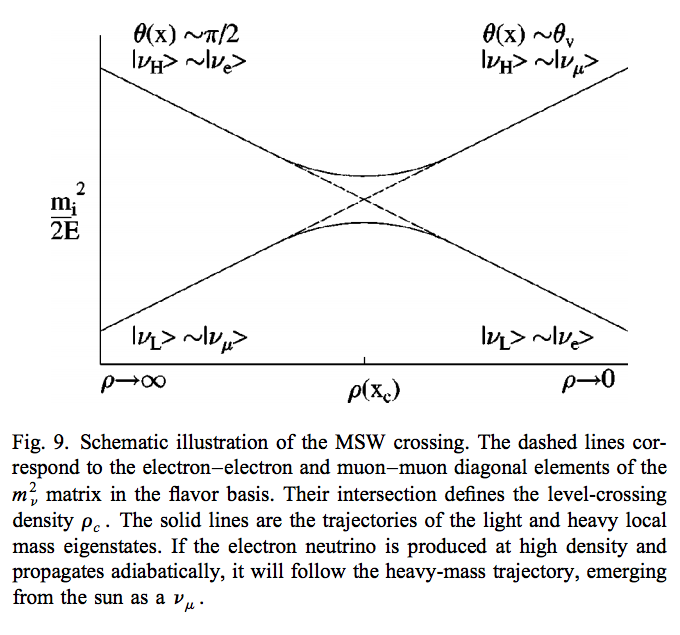
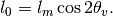
In other words, the first requirement of MSW effect is that the electrons interacts with neutrinos and makes it in a specific state that is heavy if the electron density is strong enough. Meanwhile, if the mixing angle is not that large, a level crossing could happen making the state a light state as the density becomes vacuum. The other requirement, which is obvious, is that the density change should be adiabatic, the meaning of which is the density profile of matter gently reduces to vacuum, leaving enough reaction time for the neutrinos.
The MSW effect itself can be made clear using the example of neutrino oscillations in our sun.
Small Mixing Angle
Take two flavour mixing as an example.
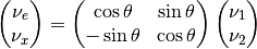
In the small mixing angle limit,
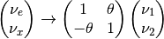
which is very close to an identity matrix. This implies that electron neutrino is more like mass eigenstate  . By we mean the state with energy
  in vacuum.
We need this intuitive picture to understand MSW effect. Electron neutrinos are almost identical to the low mass neutrino mass eigenstate. However, as we will see, due to the matter interaction, the electron flavour neutrino is corresponding to the HEAVY mass eigenstate. This is the key idea in physics of MSW effect.
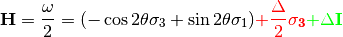
The Hamiltonian for neutinos with neutrino-matter interaction (in flavour basis) is
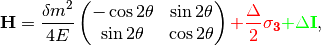
where the last term (green part) can be neglected because this term will only shift all the eigenvalues with the same amount without changing the eigenvectors.
Define a quantities like  for neutrinos (
  for antineutrinos) and
  (which might be denoted by
  in other lituratures).
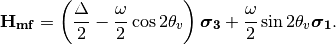
Using Pauli matrices, I can decompose this to
Note
As a reminder, .
Note
The red part is from the charged current Feynman diagram. We have a  matrix instead of an matrix like

because we rewrite this matrix with Pauli matrices and identy. Then the identities are neglected.
This can be done properly because Pauli matrice and Identy matrix form a complete basis.
In a more compact form, this Hamiltonian is
Note
Eigenvalues of  are 1 and -1 with corresponding eigenvectors

and

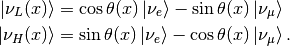
As we have mentioned, this Hamiltonian is in flavour basis. When mixing angle  , the eigenvectors are almost eigenvectors of
  which are electron neutrinos and x type neutrinos.
Interesting Limits
Before we really solve the equation of motion, some interesting limits can be shown here.
Interaction  is much larger than cacuum mixing terms. In this case, the Hamiltonian becomes diagonalized and the neutrinos will stay on it’s flavour eigenstates in the propagation.
Interaction is much smaller than vacuum mixing terms. The propagation reduces to vacuum case.
To see this effect quantitively, we need to diagonalize this Hamiltonian (Can we actually diagonalize the equation of motion? NO!). Equivalently, we can rewrite it in the basis of mass eigenstates 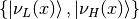 ,
,
This new rotation in matrix form is
Diagonalize Hamiltonian
To diagonilize it, we need to multiply on both sides the rotation matrix and its inverse,
The second step is to set the off diagonal elements to zero. By solving the equaions we can find the  and
and  .
.
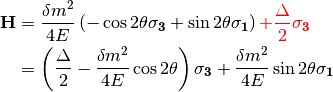
where
Set the off-diagonal elements to zero,

So the solutions are
Plug in  and
and 
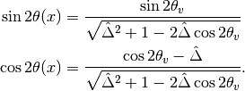
Define  with
with  , which represents the matter interaction strength compared to the vacuum oscillation.
This diagonalize the Hamiltonian LOCALLY. It’s not possible to diagonalize the Hamiltonian globally if the electron number density is not a constant.
The point is, for equation of motion, we have a differentiation with respect to position  ! So even we diagonalize the Hamiltonian, the equation of motion won’t be diagonalized. An extra matrix will occur on the LHS and de-diagonalize the Hamiltonian on RHS.
Note
As  ,
,  and vanishes. Thus the neutrino will stay on flavour eigenstates.
With the newly defined heavy-light mass eigenstates, we can calculate the propagatioin of neutrinos,

where the  comes from the fact that changing from flavor basis
  to heavy-light basis
  using
using  ,
,

only returns

We imediately know the propagation is on the heavy-light mass eigenstates under adiabatic condition WITHOUT solving the equation. The eigenvalue of these states are  and
and  . The absolute value of these solutions grow as becomes large.
Combining the two terms on RHS,

where

The only part inside  that is space dependent is the number density of the electrons . Thus we know immediately that the Hamiltonian is diagonalized if the number density is constant.
Is Adabatic Condition Valid Here?
Haxton’s paper.
Before going into the system, here is a discussion of adiabatic in thermodynamics.
From the two solutions we know there is a gap between the two trajectories. We draw a figure with electron number density as the horizontal axis and energy as the vertical axis.
Neutrino physics by Wick C. Haxton and Barry R. Holstein.
MSW Refraction, Resonance and More
Hysteresis Loops of Neutrino Oscillations Due to MSW Effect
Due to MSW effect, a system that is close to adiabaticity but not exactly adiabaticity could exhibit hysteresis effect, i.e., neutrinos going from high density region to low density region then coming back could form a hysteresis loop.
TODO
- Write down the effective potential
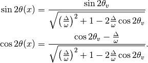
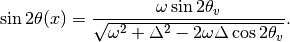
 which depends on the position. Refractive index is defined as
 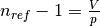 .
. - Two characteristic length:
 as the vacuum oscillation length and
  as the refraction length. As the becomes comparable resonance occurs. For small mixing angle cases, resonance happens when vacuum length is about the length of refraction.
There are three different matrix representatioins that is useful to the calculations.
- Flavor basis;
- Vacuum mass eigenstate basis;
- Instataneous mass eigenstate basis.
Basis of Hamiltonian
In vacuum mass eigenstate basis, the Hamiltonian without matter and self-interaction is easy and straightforward,
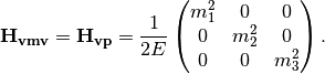
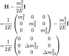
To remove the trace, we can subtract a identity matrix
The interaction in flavor basis is
To write down the Hamiltonian in vacuum mass eigenstates, we transform the interaction term to vacuum mass eigenstates by
where  is the PMNS matrix.
To write down the Hamiltonian in flavor basis, we transform the vacuum Hamiltonian to flavor basis after remove the trace, which is
We could also write down the Hamiltonian matrix in instantaneous mass eigenstates, which requires a instantaneous diagonalization.
2 Flavor Neutrino Oscillations and Matter Effect
Solar Neutrinos
Electron neutrinos are produced in the core of the sun then the neutrinos would propagate out to the surface of the sun without much difficulty. What is the predicted neutrino survival probability?
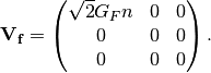
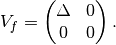
Interaction with matter plays a big role in neutrino oscillation. As shown previously, the interaction only affects (anti) electron neutrinos. In other words, the interaction term in flavor basis is
where  and
and  is the number density of the electrons. However, to do calculations, since identity matrix doesn’t change the survival probability, we can always make the hamiltonian traceless, which becomes

Constant Electron Number Density
Suppose we have an environment with constant electron number density, the term  goes away. All we have is the diagonalized new Hamiltonian
  and the eigenvalues are easily obtained which are
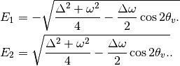
The final result for these two eigenvalues are
Meanwhile the eigenstates are denoted as  ket{nu_{c2}}`.
Two Special Cases
Two special cases,
 ;
; .
.
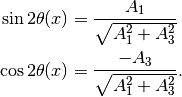
As for the survival probability for the initial condition that  , the result has the same form as the vacuum case, which is
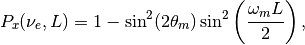
where
 is the effective mixing angle which in fact doesn’t depend on if the matter profile is constant.
Vacuum Survival Probability
As an comparison, the vacuum result is
for all electron flavor initial condition.
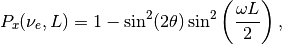
Adiabatic Limit
In some astrophysical environments the electron number density changes very slowly which means the term  is much smaller than . By intuition we would expect that this term could be dropped to the lowest order.
The eigen energies are slowing changing with the position of neutrinos,
When the term  is very small
 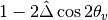 will dominate and the whole term decreases. On the other hand as becomes large,
  will dominate and the whole term grows. Mathematically we could find the region when the part
 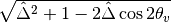 decreases and increases.
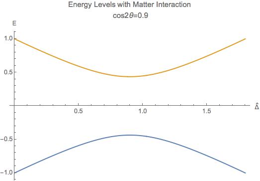
Energy Levels for MSW effect. We have the up-down symmetry since we shifted the energy by a constant to remove the identity matrix in the Hamiltonian.
The survival probability for the light neutrinos would be
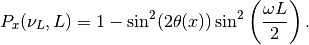
The survival probability for electron flavor neutrino is
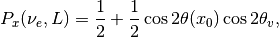
if the neutrinos are produced in dense region and the detection happens in vacuum.
Adiabatic Limit of Nuetrino Oscillations in Matter
Before we move on to higher order corrections, it would be nice to understand this phenomenon.
- The vacuum oscillation length can be extracted from vacuum oscillation survival probability. It is
 .
. - In this problem we have another energy scale which is the interaction, . Here we can define another characteristic length
 .
. - MSW resonance happens when the two character lengths are matching with each other. Another way to put it is that the term is minimized so that we have the smallest energy gap which leads to
 . Equivalently this is the relation
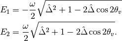
At resonance, we have
This is max mixing of the states which means that at the resonance point
Resonance conditions corresponds to a resonance density which is given by
where
 is a characteristic number density which depends on the energy mixing angles and
  of the neutrinos.
One should notice that if the condition
 is satisfied, the survival probability for
  has the same the form of vacuum oscillation survival probability for electron neutrinos. The condition is solved,
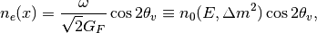
which leads to
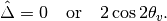
The first condition is trivial which corresponds to vacuum however the second condition $Delta = 2cos 2theta_v omega$ means the interaction oscillation length is doubled compared to resonance point.
Nevertheless, we should always remember to check what survival probability the expression is describing. Here we have survival probability for :math:`nu_L(x)`. At
 the oscillation becomes vacuum oscillation.
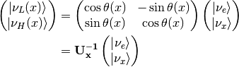
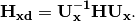
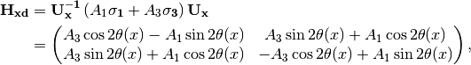
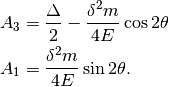
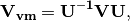
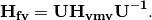
General Discussion of Matter Effect
This part is a very general discussion of the matter effect [Parke1986].
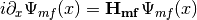
To work in flavor basis, we use the subscript  to denote the flavor basis representation with mass effect. The equation of motion in flavor basis can be written down as
where
There are three stages for neutrinos to travel from the core of the sun to vacuum.
At the core, electron neutrinos are produced. The electron flavor state should be projected onto heavy and light instantaneous mass eigenstates. What fallows is the that the propagation is adiabatic until the transition happens. As we have seen in adiabatic situation, the states will stay in heavy and light states all along the evolution if the system starts from heavy or light state,
where the heavy and light states are defined in the adiabatic situation previously. This is what happens before the passing through of the resonance.
At the resonance point, light instantaneous mass eigenstate has a probability to jump to the heavy state and vice versa. When it comes to the resonance point which is non-adiabatic propagation, the transition between the states
 and
and  will mix the heavy and light state up.
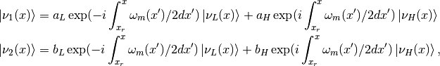
where the relations between the constants are determined using the condition that
 and
and  are orthonormal, which leads to the conclusion that
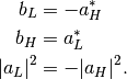
After the resonance point, the heavy and light states will continue on their adiabatic propagation.
Helpful Notes
The relation between  and
and  is given by

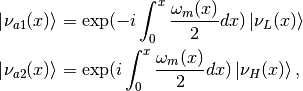
Electron neutrinos are produced in a dense region as  , which are partially transformed to other the other neutrinos due to matter and the resonance then it propagates as if it satisfies the adiabatic condition again. The initial state in terms of light and heavy state is

The final state right before the resonance is

After the resonance the state is described by the general jumping

in which the  is actually
  thus
thus
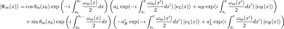
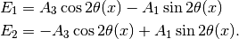
To calculate the survival probability it is easier to use flavor basis, hence we have another form of  which is
![\ket{\Psi_{m}(x)}= & \left[ \cos\theta_m(x_0) \exp\left( -i \int_{x_0}^{x_{r}} \frac{\omega_m(x')}{2} dx' \right) a_L \exp( -i \int_{x_r}^x \frac{\omega_m(x')}{2}dx' ) \right. \\
& \left. - \sin\theta_m(x_{0}) \exp\left( i \int_{x_0}^{x_{r-}} \frac{\omega_m(x')}{2} dx' \right) a_H^* \exp( -i \int_{x_r}^x \frac{\omega_m(x')}{2}dx' ) \right] \ket{\nu_L(x)}\\
& + \left[ \cos\theta_m(x_0) \exp\left( -i \int_{x_0}^{x_{r}} \frac{\omega_m(x)}{2} dx \right) a_H \exp( i\int_{x_r}^x \frac{\omega_m(x')}{2}dx' ) \right. \\
& \left. + \sin\theta_m(x_{0}) \exp\left( i \int_{x_0}^{x_{r-}} \frac{\omega_m(x)}{2} dx \right) a_L^* \exp( i\int_{x_r}^x \frac{\omega_m(x')}{2}dx' ) \right] \ket{\nu_H(x)} \\
=& \left[ \cos\theta_m(x_0) \exp\left( -i \int_{x_0}^{x_{r}} \frac{\omega_m(x)}{2} dx \right) a_L \exp( -i \int_{x_r}^x \frac{\omega_m(x')}{2}dx' ) \right. \\
& \left. - \sin\theta_m(x_{0}) \exp\left( i \int_{x_0}^{x_{r-}} \frac{\omega_m(x)}{2} dx \right) a_H^* \exp( -i \int_{x_r}^x \frac{\omega_m(x')}{2}dx' ) \right] ( \cos\theta_m(x)\ket{\nu_e} - \sin\theta_m(x)\ket{\nu_x} )\\
& + \left[ \cos\theta_m(x_0) \exp\left( -i \int_{x_0}^{x_{r}} \frac{\omega_m(x)}{2} dx \right) a_H \exp( i\int_{x_r}^x \frac{\omega_m(x')}{2}dx' ) \right. \\
& \left. + \sin\theta_m(x_{0}) \exp\left( i \int_{x_0}^{x_{r-}} \frac{\omega_m(x)}{2} dx \right) a_L^* \exp( i\int_{x_r}^x \frac{\omega_m(x')}{2}dx' ) \right] ( \sin\theta_m(x)\ket{\nu_e} + \cos\theta_m(x)\ket{\nu_x})](_images/math/ac79874b5ec44cf2151b807a2d5f56f23aa7b1b2.png)
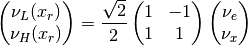
Since  ,
,  and
and  are real while
  and
and  are complex, survival amplitude of electron neutrinos is given by
![&\braket{\Psi_m(0)}{\Psi_m(x)} \\
= & \braket{\nu_e}{\Psi_m(x)} \\
= & \left[ \cos\theta_m(x_0) \exp\left( -i \int_{x_0}^{x_{r}} \frac{\omega_m(x')}{2} dx' \right) a_L \exp( -i \int_{x_r}^x \frac{\omega_m(x')}{2}dx' ) \right. \\
& \left. - \sin\theta_m(x_{0}) \exp\left( i \int_{x_0}^{x_{r}} \frac{\omega_m(x')}{2} dx' \right) a_H^* \exp( -i \int_{x_r}^x \frac{\omega_m(x')}{2}dx' ) \right] \cos\theta_m(x) \\
& + \left[ \cos\theta_m(x_0) \exp\left( -i \int_{x_0}^{x_{r}} \frac{\omega_m(x')}{2} dx' \right) a_H \exp( i\int_{x_r}^x \frac{\omega_m(x')}{2}dx' ) \right. \\
& \left. + \sin\theta_m(x_{0}) \exp\left( i \int_{x_0}^{x_{r}} \frac{\omega_m(x')}{2} dx' \right) a_L^* \exp( i\int_{x_r}^x \frac{\omega_m(x')}{2}dx' ) \right] \sin\theta_m(x) \\
=& A_L \exp\left( -i \int_{x_r}^{x} \frac{\omega_m(x')}{2} dx' \right) + A_H \exp\left( i\int_{x_r}^x \frac{\omega_m(x')}{2}dx' \right),](_images/math/44c20c91968a060ad90676e9ea7f42abb1035cd1.png)
where the coefficients are
![A_L(x) & = \cos\theta_m(x) \left[ a_L\cos\theta_m(x_0) \exp\left( -i\int_{x_0}^{x_r} \frac{\omega_m(x')}{2} dx' \right) - a_H^*\sin\theta_m(x_0) \exp\left( i \int_{x_0}^{x_r} \frac{\omega_m(x')}{2}dx' \right) \right] \\
A_H(x) & = \sin\theta_m(x) \left[ a_H \cos\theta_m(x_0) \exp\left( -i \int_{x_0}^{x_{r}} \frac{\omega_m(x')}{2} dx' \right) + a_L^*\sin\theta_m(x_{0}) \exp\left( i \int_{x_0}^{x_{r}} \frac{\omega_m(x')}{2} dx' \right) \right] .](_images/math/d24aa52a771595af82abb3e66254098f06747908.png)
The detection is in a region where matter density is very small, thus we use  which means the effective mixing angle becomes vacuum mixing angle. The probability is the square of the amplitude,
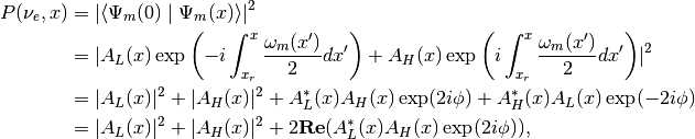
where  is defined as
Note that for any complex number  ,
,

which means that the previous result can be simplified to

with the definition that  is the argument of $A_L^*(x)A_H(x)$.
However the coefficients and are still not known yet. The trick is to average over the detection and production position. The average over removes the  term due to the dependent of for and averages
  to
to  , which results in
Applying the condition that  , the probability becomes

where  is the argument of
  and is
  .
.
The average over production removes the last part.
Notice that in fact the detection happens in vacuum, which means  .
.

This means that the adiabatic result is of the form
Define a transition probability at resonance
which can be determined by the Landau-Zener transition analytically (first order) to the first order.
| [Parke1986] | Parke, S. J. (1986). Nonadiabatic Level Crossing in Resonant Neutrino Oscillations. Physical Review Letters, 57(10), 1275–1278. doi:10.1103/PhysRevLett.57.1275 |
Refs and Notes
- Wolfenstein, L. (1978). Neutrino oscillations in matter. Physical Review D, 17(9), 2369–2374. doi:10.1103/PhysRevD.17.2369
- Wolfenstein, L. (1979). Neutrino oscillations and stellar collapse. Physical Review D, 20(10), 2634–2635. doi:10.1103/PhysRevD.20.2634
- Parke, S. J. (1986). Nonadiabatic Level Crossing in Resonant Neutrino Oscillations. Physical Review Letters, 57(10), 1275–1278. doi:10.1103/PhysRevLett.57.1275
- Bethe, H. A. (1986). Possible Explanation of the Solar-Neutrino Puzzle. Physical Review Letters, 56(12), 1305–1308. doi:10.1103/PhysRevLett.56.1305